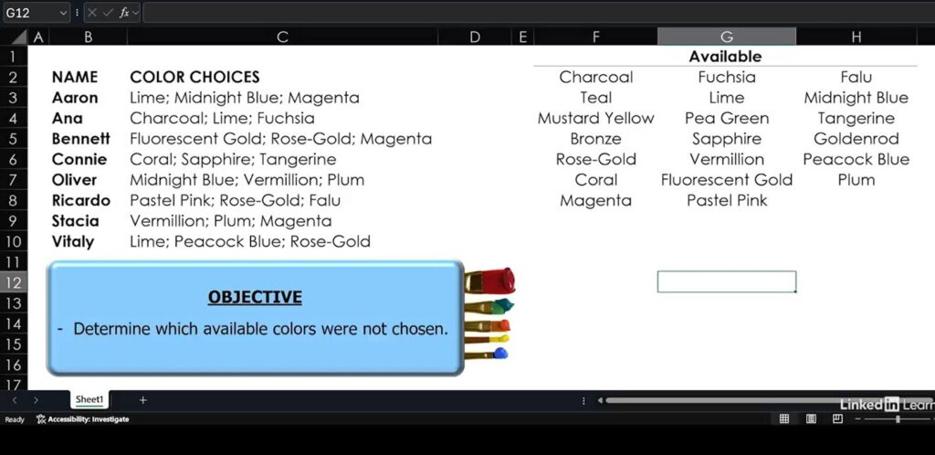
Welcome to the Excel challenge by Oz de Soleil posts on Friday 6 September 2024! We’re diving into a real-world scenario, and my approach may differ from the conventional paths. The challenge revolves around two lists of colours: one is a list of colours that people have picked, and the other contains the available colours. Your task? Find out which colours haven’t been picked by anyone.
At first glance, this seems straightforward. Many solutions have been provided, and they’re all likely to work. Excel expert Oz du Soleil even has a video explainer on the topic. However, I’d like to offer a slightly different perspective.

Step 1: Understanding the Problem Through Common Sense.
When approaching this challenge, let’s start with common sense. By that, I mean everyday logic–something we all use unconsciously. For example, think about preparing for a dinner party. You have a recipe, and before you head to the store, you check what ingredients you already have at home. What you’re left with is a list of things you need to buy, i.e., the difference between two lists.
Similarly, for this challenge, you’re dealing with two lists of colors–one of picked colours and one of available colors. The goal is to identify which colours are in the available list but not in the picked list. Simple enough, right?
Step 2: Recognizing the Lists.
One hurdle people often face is that the data doesn’t *look* like traditional lists–it might be laid out differently. But the moment you realize that they are, in fact, lists, you’re already halfway there. It’s all about perspective.
Now, once you’ve recognized them as lists, the next task is to convert these blocks of data into something we can work with–tables. Whether you use VBA, Power Query, or manual methods, the goal is to turn these blocks into tables.
Step 3: Eliminating Items Using a Join.
If you’ve worked with Power Query, you probably know how to eliminate items from one list based on another. Through a data model, you can easily filter out the colours that haven’t been picked. This is where the “join” function comes into play. You create a relationship between the two tables–one for picked colours and one for available colours–and filter out the results.
By joining the two lists, we get the answer: the colors that haven’t been picked.
Step 4: Why This Approach is Different.
Many solutions jump straight into using formulas or tools like Power Query. While effective, those methods often involve specific features or functions. My approach starts from common sense and works up from there, ensuring that you understand the problem in its simplest form–without needing to rely on advanced Excel features unless necessary.
Instead of relying on Power Query or formulas as a crutch, we break the problem down into basic, reusable steps:
1. Recognize that we are comparing two lists.
2. Convert those lists into tables.
3. Use a simple join to filter the data.
This process not only solves the problem but can also be adapted to many other data challenges without depending on advanced tools.
Step 5: The Bigger Picture.
This approach isn’t just about solving an isolated task in Excel; it’s about building a more resilient method. By focusing on common sense and principles like joining tables, you can create solutions that go beyond just this challenge. In fact, I’ve applied this in broader business contexts, like integrating data from multiple departments into a central database for organization-wide analysis.
In conclusion, sometimes the most powerful Excel solutions come from thinking beyond the formula.
You’ve been listening to a podcast by Hiran de Silva. Red by Bill.


Add comment